Mapping bomb shelters in Be'er-Sheva, IL

Update from March 21, 2020

I’ve been wanting to return to this post and make this map more interactive. As a matter of fact it was easier than I thought, I just never got around to doing it. I won’t be going through the code for the leaflet map below but will leave it for whoever would like to review it:

library(leaflet)
library(magrittr)
readr::read_csv("shelters.csv") %>% 
leaflet() %>% 
  addTiles() %>% 
  setView(34.7913, 31.25181,zoom = 13) %>% 
  addCircles(radius = 4, color = "red", fill = TRUE)

Original post

I’ve been wanting to learn how to use maps in R for a while before creating the map in this post. Seeing dataframes with longitude and latitude coordinates on various occasions on #Tidytuesday encouraged me to do so.
A day before this visualizaiton, I discovered our municupality’s open access data website. In this website you can find various datasets like street light coordinates, bomb shelters spread out in the city and more. A day after discovering it Israel, the country I live in, was fired missiles at. I decided to take the opportunity and map some of the shelters around my house. You know, just in case.

Let’s begin with the packages (📦) we’ll need:

#for data manipulation
library(tidyverse)
#for a nice map
library(ggmap)
#for reading and working with .geojson file
library(geojsonio)
library(sp)
#for integrating a nice font
library(extrafont)

Loading and tidying the data

I initially tried using the .csv file they have on their webiste but I was having too much trouble with the Hebrew so I decided to try and work with the geojsonio package. I had no idea how to work with a .geojson file or frankly how to work with maps in general. To my save, i found this incredible blog by John Johnson to help me transform a ‘geomjson’ file to a dataframe you can work with.

Let’s begin:

#read the .geojson file
my_geojson <- "shelters.geojson"
#convert the .geojson file to an sp object
data_json <- geojson_read(my_geojson, what = "sp")
#now we can convert it to a nice data frame
shelters <- as.data.frame(data_json)
#last tidying of the column names
names(shelters)[6:7] <- c("long", "lat")

What we did was load the geojson file, read it as an ‘sp’ object and then turn it into to a dataframe. I changed the names so that it’ll be easier to read the columns. we could also use dplyr::rename but I liked the base R function Johnson used in his blog so I’ll stick with that.
let’s look at the top 3 observations of our new data frame:

##       long      lat name קוד_ס elc group_ F_צוות
## 1 34.80821 31.25902  ג/2    17  יש      0       
## 2 34.80789 31.25980  ג/1    17  יש      0       
## 3 34.80937 31.25925 ג/25    17  יש      0

Ugh, well the names weren’t read well into R. While this isn’t a big issue to resolve, I don’t find it necessary for the final piece. the names of the shelters are anyway in Hebrew and only represnt a letter and some sort of number (for e.g, A/23, only in Hebrew). Therefore we’ll leave it as is since what I’m interested in is the longitude and latitude coordinations and for that we don’t need the character column.

Retrieving the map

So we have our data frame with long and lat points, let’s get our map. I want a map that can be readable in terms of streets and roads, therefore I’ll give the ggmap package a try¹. Google requires you to register in order to recieve an API key to pull maps to plot. Unfortunately I won’t cover how to regiser in this blog post but I’m sure you can find plenty of tutorials addressing it online.
Let’s get Be’er-Sheva’s map:

b7_map <- get_map(location = c(34.7913 , 31.25181), 
              zoom = 13, scale = 2, maptype = "roadmap")

What we did here was use the get_map function to pull the map according to the long and lat coordinates I gave it of Be’er-Sheva. You should first pass the longitude and then the latitude in the location argument. In addition you can change other features such as the zoom level, the maptype and more as we saw here (See ?get_map for more info).

Plot

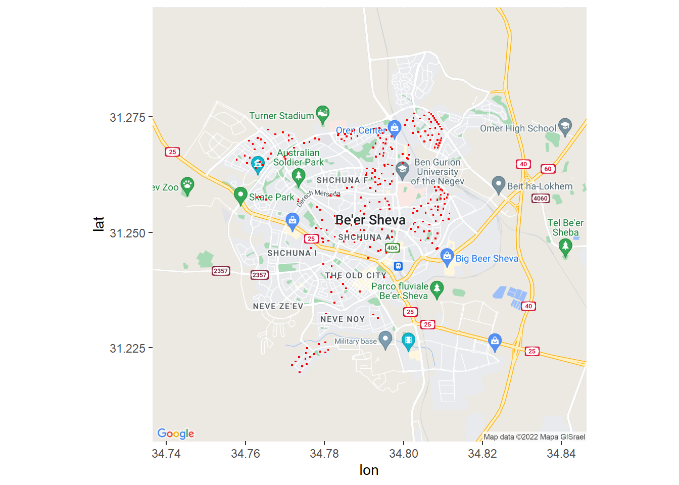
Now that we have our data set ready and the map as an object we can go on to plot it. ggmap extends ggplot features so we can run the data frame smoothly into the ggmap function:

ggmap(b7_map)+
  geom_point(shelters, mapping = aes(long,lat),
            color = "red", size = 0.3, shape = 15)

What we did was pass the b7_map as an object into the ggmap function and add a geom, in this case geom_point representing our shelter coordinates. However, this map doesn’t really help me in a time of need since it doesn’t show my address clearly.

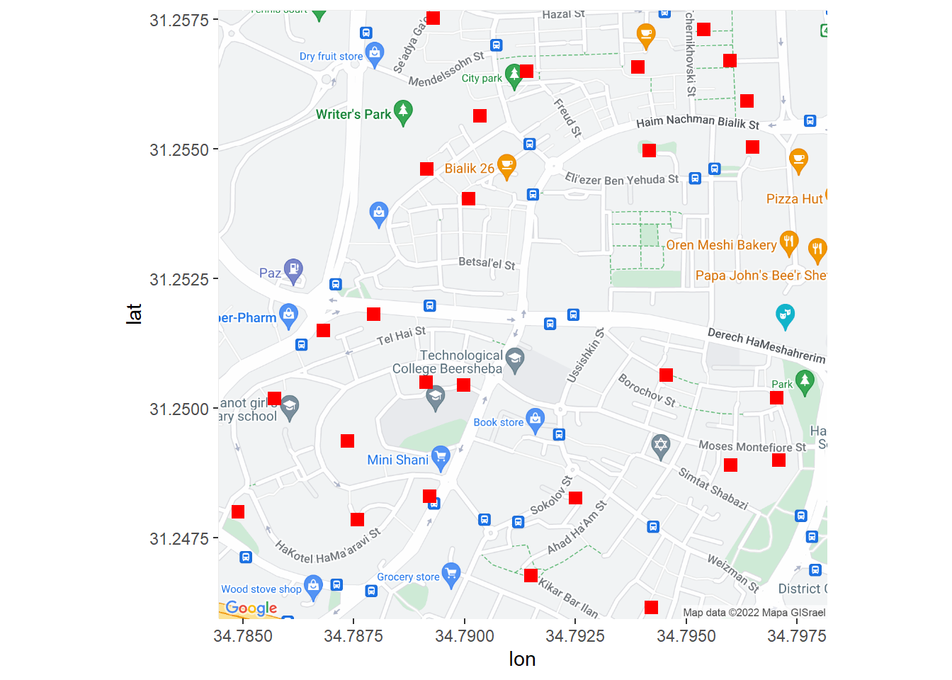
Let’s try zooming in so that we can see what we’re looking at:

#retreiving a new map with a greater `zoom`
b7_map_zoom <- get_map(location = c(34.7913 , 31.25181), 
                    zoom = 16, scale = 2, maptype = "roadmap")

p <- ggmap(b7_map_zoom)+
geom_point(shelters, mapping = aes(long,lat), color = "red",
           size = 3, shape = 15)
p

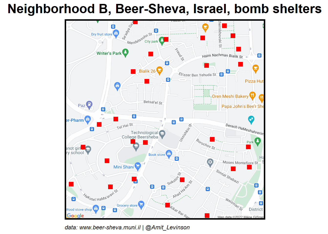
Much nicer and clearer. Using the zoom option in get_map enables to center more on where I want. Great, this shows me some bomb shetlers I have around me in a time of need. Let’s add some fine tuning for our theme:

p+  
#for the title, caption and removing the X and Y axis
  labs (title = "Neighborhood B, Beer-Sheva, Israel, bomb shelters",
        x = NULL, y = NULL,
        caption = "data: www.beer-sheva.muni.il | @Amit_Levinson")+
  theme_minimal()+
  theme(text = element_text(family = "Microsoft Tai Le"),
    #Changing the position of the title
    plot.title = element_text(hjust = 0.5, size = 20, face = "bold"),
    axis.text = element_blank(),
    plot.caption = element_text(size = 9, face = "italic", hjust = 0),
    panel.border = element_rect(color = "black", size=2, fill = NA)
  )

Perfect, I can now save the plot and distribute it if someone needs it.

ggsave("shelters_b_eng.png", width = 8, height = 8)