Distances to Golda Ice-Cream Locations in Israel
By Amit Grinson in R
February 10, 2021
What’s this all about
This past November I participated several times in the #30DaysMapChallenge, a daily mapping visualization challenge. While I was satisfied with what I came up with, my main outcome was that I have no idea how to work with maps. Well, to say it differently, I was able to fiddle around and hit home eventually, but my knowledge of Coordinate Referencing Systems (CRS) and other important features was limited. For that purpose, I knew I’ll be back to explore some additional geographic data, leading to the following blog post.
In this blog post I’ll explore Golda Ice-cream locations throughout Israel. My wife and I came across Golda one day and were happily surprised when first tasting it: the ice-cream was fantastic, especially compared to other ice-cream shops we previously visited. Golda has a plethora of ice-cream flavors including fantastic Sorbets, chocolate pretzel, salted cashew, vanilla chocolate pistachio and more. Also, they have this really amazing pretzel sauce you can drizzle on top, what a treat!
 Golda’s delicious ice-cream flavors. Source: [Golda Facebook page](https://www.facebook.com/GLIDAGOLDAISRAEL)
To follow through with my motivation to learn more about maps and as a tribute to their great ice-cream I decided to explore Golda’s ice-cream locations. More specifically, we’ll be looking at distances from various points in the country to the nearest ice-cream location. Following a short overview of the data collection and ice-cream locations throughout Israel I will address the utmost important question pertaining distances and Golda locations:
Where do you not want to be if you want an ice-cream now?
I will say that I have no affiliation nor received any compensation for this post. I’m genuinely writing this as a means to learn about maps by exploring ice-cream locations. Stick with me if you want to learn about the nearest ice-cream shop to you.
Before we begin, a big thank you goes to Dominic Roye’s blog post on distances from the shore in Iceland for inspiration and practical help with the code. On a more theoretical level, I enjoyed and learned from Michael Dorman’s ‘Using R for Spatial Data Analysis’ materials from a workshop he gave. I highly recommend exploring both.
In contrast to previous blog posts of mine this one will not display code or raw data. However, I invite you to explore the full source code to learn what’s done under the hood.
Golda location information
I web-scraped Golda’s website to extract relevant information such as street addresses in Hebrew. To get exact locations I geocoded those street addresses using the {ggmap} R package, extracting corresponding latitude & longitude coordinates for each scraped address. I then queried the received longitude and latitude for Golda’s addresses in English to validate the information initially extracted.
Essentially, I geocoded the data twice. Any addresses in English that didn’t match the Hebrew ones I manually checked for the correct location. I identified about 2-3 locations that the extracted information was 250 meters off. Some locations might still not be exact, but overall I think we’re good to go. You can explore the scraping script and complete dataset with English locations for further info.
Our Golda ice-cream dataset looks as follows:
We have a total of 79 locations throughout Israel. Each row represents a store, the city and street it’s located in, their phone number and a corresponding longitude and latitude point. A few stores on the website were noted as currently closed, but for the sake of this post will treat them like all others.
Let’s see where they are across Israel:
A quick overview of our map shows that majority of Golda locations are in the Tel-Aviv metropolitan area (center of Israel). Other locations are scattered across the country with several in the north and a few down south. You can also hover over a location to learn where exactly is it located.
Measuring distances
We (well, I) want to calculate the distances to each Ice-cream location from various points on the map. Doing so requires us to project our map to a different coordinate reference system than the current. That is, our current CRS uses geographic coordinates that account for earth’s curvature, when we want a flat surface to measure distances. Think of it as cutting open a basketball, flattening it and then measuring a distance from two points.
Furthermore, We want to measure distances from various locations on the map to the nearest Golda ice-cream location. However, distance from ‘various locations’ is somewhat abstract; we want the distance from something a little more specific. To tackle that query, we’ll divide the geographical area of Israel into grids.
Grids… What? Let’s have a look:
Show Code
theme_set(theme_void()+
            theme(text = element_text("IBM Plex Sans"),
                  plot.title = element_text(color = "#0C0C44", face = "bold")))

p1 <- ggplot(isr_map_sf)+
  geom_sf()

p2 <- ggplot(grid)+
  geom_sf()

p1+p2+
  plot_annotation(
    title = "Map of Isreal (left) and map cut into 2km<sup>2</sup> areas (right)",
    theme = theme(plot.title = element_markdown(size = 12)))
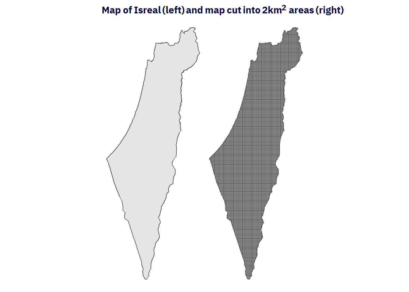
On the left we have our map of Israel, and on the right the same map after we ‘cut’ it horizontally and vertically. Each grid represents a square polygon (except those on the borders) with specific geographic references to plot it, creating a 2 squared kilometers area (2km$^2$). We can measure the distance from the center of each 2km$^2$ grid to the nearest ice-cream location.
In practical terms, here’s an example of distances from one random grid to a few random Golda locations:
Show Code
# Create a sampled dataframe
dataum <- data.frame(
  geometry = st_geometry(golda_projected[3:9,]),
  location_grid = st_centroid(rep(grid_wgs[350],7)))


# Our data points projected to a
data_lines <- map_dfc(dataum, ~ st_transform(.x, crs = 2039))

sample_data <- data_lines %>%
  map_dfc(~ st_transform(.x, crs = 4326) %>% st_coordinates(.x)) %>%
  map_dfc(as.data.frame) %>%
  set_names(c("golda.x","golda.y", "us.x" ,"us.y")) %>%
  cbind(distance = map2_dbl(data_lines$geometry, data_lines$geometry.1,  st_distance),
        location_polygon = st_transform(data_lines$geometry.1, crs = 4326)) %>%
  mutate(relevant = ifelse(distance == min(distance), "yes", "no"),
         distance = ifelse(relevant == "yes", paste0(round(distance/1000, 0), "km"), round(distance/1000, 0)))

point_labels <- data.frame(x = c(34.802,34.95968, 34.79946),
                           y = c(30.04696, 29.54952, 31.23412),
                           label = c("Example grid", "Nearest Golda", "Golda locations"))

ggplot(isr_map_sf)+
  geom_sf()+
  geom_point(data = sample_data,mapping= aes(x = golda.x, y = golda.y, color = relevant), size = 1.2)+
  geom_sf(data = grid_wgs[350], aes(geometry = geometry), fill = "red", color = "red")+
  geom_spatial_segment(data = sample_data, mapping = aes(x = us.x, xend = golda.x, y = us.y, yend = golda.y, linetype = relevant, color = relevant), show.legend = FALSE)+
  geom_spatial_text_repel(data = sample_data, mapping = aes(x = golda.x,  y = golda.y, label = distance, color = relevant), crs = 4326, hjust = 0.5, size = 3.5)+
  geom_text_repel(data = point_labels, mapping = aes(x = x, y = y, label = label), xlim = c(35.5,36), point.padding = 0.1,  arrow = arrow(length = unit(0.015, "npc"), type = "closed"), segment.linetype = 8, color = "gray55", segment.color = "gray80", size = 3)+
  scale_color_manual(values = c("yes" = "red", "no" = "gray60"))+
  scale_linetype_manual(values = c("dashed","solid"))+
  xlim(34,36)+
  coord_sf(clip = "off")+
  guides(color = "none")+
  labs(title = "Finding the nearest Golda location for each grid")+
  theme(plot.title = element_text(size = 13, hjust = 0.5))
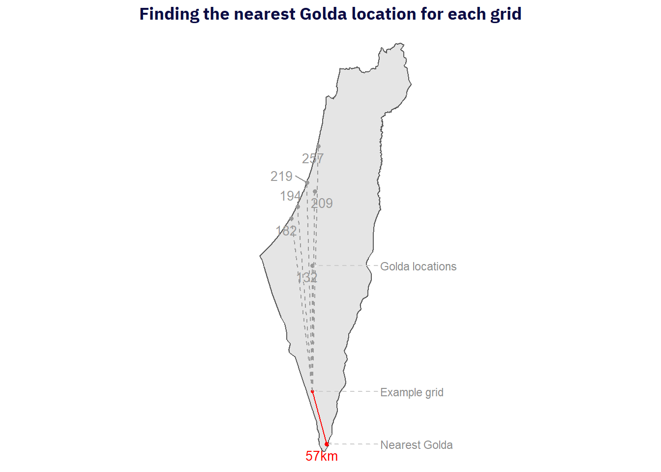
Our small square represents a 2km$^2$ area somewhere in southern Israel. The lines and corresponding values indicate the distance to each ice-cream location from our example grid. To be specific, I measure the air distance from the center of a grid cell to the various locations. In the above graph our sampled grid is connected with a red line to the nearest ice-cream location located in Eilat, 57km away.

Where’s Our Ice-cream
Once we understand how each grid’s nearest ice-cream location distance is found we can measure accordingly for all grids. Following that we can create a map of our grid cells filled with color indicating the distance to the nearest Golda ice-cream location:
Show Code
# Commented out and loaded as an rds instead. Calculate distances:
# distances <- st_distance(golda_meters, st_centroid(grid)) %>%
# as_tibble()

# Loaded as rds for faster rendering
distances <- read_rds("rds/distances.rds")

golda_distances <- data.frame(
  # We want grids in a WGS 84 CRS:
  us = st_transform(grid, crs = 4326),
  # Extract minimum distance for each grid
  distance_km = map_dbl(distances, min)/1000,
  # Extract the value's index for joining with the ice-cream location info
  location_id = map_dbl(distances, function(x) match(min(x), x))) %>%
  # Join with the ice-cream table
  left_join(golda_projected, by = c("location_id" = "id"))


# We don't evaluate this as I saved it as a widget instead.
# ice_cream_icon <-  makeIcon("ice-cream.png", iconWidth = 6, iconHeight = 8)

# Decrease size of ice-cream icons
ice_cream_icon <- makeIcon("https://upload.wikimedia.org/wikipedia/commons/2/2c/Ice-cream-solid.svg", iconWidth = 6, iconHeight = 10)

# Bin ranges for a nicer color scale
bins <- c(0,5,15,30,50,70)
# Create a binned color palette
pal <- colorBin(c("#FF1554", "#FF3C70", "#FF7096", "#FFA4BC", "#FFE5EC"), domain = golda_distances$distance_km, bins = bins, reverse = TRUE)

#Pink colors more variance:
# c("#FF1554", "#FF3C70", "#FF7096", "#FFA4BC", "#FFE5EC")

    #ff084a
# Function to create the labels indicating distances
make_label_distances <- function(km, street, city){
  glue("
  <div style='text-align:left;'>
  You are <span style='font-size:13px;'><b>{round(km, 1)}</b></span> km from the nearest location at:</div>
  <div style='text-align:right;'>
       {street}, {city}</div>") %>%
    HTML()}
# Create the labels
ice_cream_labels <- pmap(list(golda_distances$distance_km, golda_distances$street,golda_distances$city), make_label_distances)

full_map <- leaflet() %>%
  addTiles() %>%
  addMarkers(data = golda_projected, icon = ~ice_cream_icon, group = "Ice-cream locations") %>%
  addPolygons(data = golda_distances[[1]], fillColor = pal(golda_distances$distance_km), fillOpacity = 0.8, weight =0,
              opacity =1, color = "transparent", group = "Distances", popup = ice_cream_labels,
              highlight = highlightOptions(weight = 2.5, color = "#666", bringToFront = TRUE, opacity= 1),
              popupOptions = popupOptions(autoPan = FALSE,closeOnClick = TRUE, textOnly = T)) %>%
   addLegend(pal = pal, values = (golda_distances$distance_km), opacity = 0.8,
                         title = "Distance (Km)", position= "bottomright") %>%
  addLayersControl(overlayGroups = c("Ice-cream locations", "Distances"),
                   options = layersControlOptions(collapsed = FALSE))

# Save the widget to use as an iframe:
# htmlwidgets::saveWidget(full_map, "widgets/full_map.html")
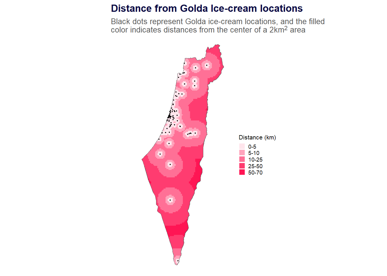
Beautiful! Well, mainly for those living near ice-cream locations.
The main conclusion is you don’t want to be stuck somewhere in southern Israel or south of the dead sea with a sudden craving for ice-cream. We also see that similar to before, those living in the Tel-Aviv metropolitan area are safe with a Golda location near by.
I’ve added a twist to the map in which you can click on a grid cell to see how far is the nearest ice cream location. The distance is measured from the center of a grid so we’ll treat the grid cell as one unit.
We could also level up the map and have the distance measured from a specific location the user clicks on, not a whole grid cell. For that we’ll need something reactable such as an interactive web app (e.g. R Shiny) providing exact distances from a point clicked on the map. It seems pretty straight forward but for the purpose of the post I found the above appropriate and a great learning experience.
Static maps
Version 1
We can visualize it on a static map enabling us to easily share it as an image:
Show Code
# Using the interactive original object we can create a
# static map:
golda_distances <- data.frame(
  us = st_transform(grid, crs = 4326),
  # Extract minimum distance for each grid
  distance_km = map_dbl(distances, min)/1000,
  # Extract the value's index for joining with the ice-cream loc info
  location_id = map_dbl(distances, function(x) match(min(x), x))) %>%
  left_join(golda_projected, by = c("location_id" = "id")) %>%
  mutate(binned_colors = cut(distance_km, breaks = c(70,50,25,10,5,0)))

pink_palette <- c("#FF1554", "#FF3C70", "#FF7096", "#FFA4BC", "#FFE5EC")


ggplot(golda_distances, color = "gray55")+
  geom_sf(data = isr_map_sf, aes(geometry = geometry))+
  geom_sf(aes(geometry = geometry.x, fill =  binned_colors), color = NA)+
  geom_point(golda_locations, mapping = aes(x = lon, y= lat), size = .3)+
  scale_fill_manual(name = "Distance (km)", values = rev(pink_palette),
                    labels = c("0-5", "5-10", "10-25", "25-50", "50-70"))+
  xlim(33.7,36)+
  labs(title = "Distance from Golda Ice-cream locations", subtitle = "Black dots represent Golda ice-cream locations, and the filled<br>color indicates distances from the center of a 2km<sup>2</sup> area")+
  # labs(caption = "Data: Golda | @Amit_Levinson")+
  theme_void()+
  theme(plot.title = element_text(color = "#0C0C44", face = "bold", size = 13),
        plot.title.position = "plot",
        plot.subtitle = element_markdown(color = "gray35", size = 10),
        # plot.caption = element_text(color = "gray55", hjust = 1, size = 6, face = "italic"),
        # plot.margin = margin(3,4,0,4,"mm"),
        legend.title = element_text(size = 8),
        legend.text = element_text(size = 7),
        legend.key.size = unit(3,"mm"))
Version 2
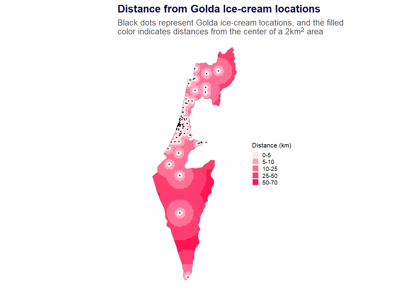
Considering the geo-political issues in Israel, which I won’t elaborate here, I’ll share another map with different borders. These borders better reflect the feasibility of individuals to access these locations since people living in, say, Gaza (plotted in previous maps), cannot access any of the locations.
Show Code
# Israel map
isr_map_rds_raw <- readRDS("maps/00_Israel_0_sf.rds")
# write_rds(grid_rds, "rds/grid_green.rds")
grid_rds <- read_rds("rds/grid_green.rds")
# write_rds(distances_rds, "rds/distances_green.rds")
distances_rds <- read_rds("rds/distances_green.rds")

golda_distances_rds <- data.frame(
  us = st_transform(grid_rds, crs = 4326),
  # Extract minimum distance for each grid
  distance_km = map_dbl(distances_rds, min)/1000,
  # Extract the value's index for joining with the ice-cream loc info
  location_id = map_dbl(distances_rds, function(x) match(min(x), x))) %>%
  left_join(golda_projected, by = c("location_id" = "id")) %>%
  mutate(binned_colors = cut(distance_km, breaks = c(70,50,25,10,5,0)))

ggplot(golda_distances_rds)+
  geom_sf(data = isr_map_rds_raw, color = "gray55")+
  geom_sf(aes(geometry = geometry.x, fill =  binned_colors, color = "black"), color = "transparent")+
  geom_point(golda_locations, mapping = aes(x = lon, y= lat), size = .3)+
  scale_fill_manual(name = "Distance (km)", values = rev(pink_palette), labels = c("0-5", "5-10", "10-25", "25-50", "50-70"))+
  xlim(33.7,36)+
  labs(title = "Distance from Golda Ice-cream locations", subtitle = "Black dots represent Golda ice-cream locations, and the filled<br>color indicates distances from the center of a 2km<sup>2</sup> area")+
  # labs(caption = "Data: Golda | @Amit_Levinson")+
  theme_void()+
  theme(plot.title = element_text(color = "#0C0C44", face = "bold", size = 13),
        plot.title.position = "plot",
        plot.subtitle = element_markdown(color = "gray35", size = 10),
        # plot.caption = element_text(color = "gray55", hjust = 1, size = 6, face = "italic"),
        # plot.margin = margin(3,4,0,4,"mm"),
        legend.title = element_text(size = 8),
        legend.text = element_text(size = 7),
        legend.key.size = unit(3,"mm"))
Conclusion
All this talk about ice-cream sure got me craving for some. I hope I didn’t instill too much ice-cream craving in you following this post, but at least now you know where to find the nearest location. I also invite you to explore the full source code or play with the data yourself.
Although a short post, I’ve learned a plenty on using maps, distances and reference systems. From a technical level it required learning about transitioning from various reference systems, calculating distances, understanding what occurs under the hood and learning how to interactively display the final result. While I definitely still don’t know enough about working with spatial data in R, I feel like I don’t know a little less after completing this blog post.
I hope you enjoyed this post and it helps you find the nearest ice-cream location next time you’re subject to an ice-cream frenzy!
- Posted on:
- February 10, 2021
- Length:
- 13 minute read, 2683 words
- Categories:
- R
- Tags:
- maps rvest interactive