R vs Python — Live Stream Analysis
Questions and answers from the live stream of an R vs Python data analysis
By Amit Grinson in R
June 2, 2022
A few months ago Tal Mizrachi (The famous Analysis Paralysis) & I live streamed an R vs Python data analysis session (in Hebrew). We took the dogs of Zurich dataset, formatted it a bit, added a random DOB column and wrote down a few questions we answered during the live stream, each with his own tool.
Besides it being a great experience collaborating with Tal, I think the questions overall touched on various aspects of our day-to-day data analysis flow. I initially
hosted the questions and answers on a GitHub page but realized they got lost in the abyss called ‘internet’. Instead, I am journalizing it on my website for future me as I pick up Python and others who want to practice their analysis skills. If you liked it, came up with a different solution or just want to share how much you love Python R, do reach out to either one of us and let us know. We’d love to hear more about your experience!
How should you read this post?
My recommendation is to first try solving the questions yourself. You can find the data-files in the link below:
Great, now that you have the data, answer the following questions with any tool you’d like. Once you have the solutions you can check them with our solutions below (just click on the question). If you’re struggling you can use the output from our answers as a hint before viewing the answer in the code chunks.
The Questions
1. Load the files into memory and combine them into a single Dataframe
2. Describe the data using a summary function of sort
5. Who (owner) has dogs with the largest age gap between them? What’s the gap value?
6. Save the Dataframe into an excel file where each sheet is a different age-group of owners
The Answers
The following section has the answers to the questions in both Python (by Tal) and R (by me). For each question you’ll find the answers in code, an output of the code and a follow up explanation for the R code or procedure we took. The code is collapsed and hidden, so just click to see it.
1. Load the files into memory and combine them into a single Dataframe
Python
import pandas as pd
import numpy as np
import os
import matplotlib.pyplot as plt
import seaborn as sns
all_files = []
for file in os.listdir("split_data/"):
    if not file.endswith("csv"):
        continue
    all_files.append(pd.read_csv("split_data/"+file))

df = pd.concat(all_files, ignore_index=True)

df
##       owner_id    age gender  ...  dog_gender    dog_color     dog_dob
## 0       124913  41-50      w  ...           m    saufarben  1996-11-10
## 1        84494  61-70      w  ...           w  schwarz/rot  1997-08-10
## 2        85293  81-90      w  ...           w  beige/weiss  1997-09-10
## 3        80204  51-60      w  ...           m   dreifarbig  1998-08-10
## 4        80399  61-70      w  ...           m     tricolor  1998-08-10
## ...        ...    ...    ...  ...         ...          ...         ...
## 7150    135725  31-40      w  ...           w   gelb/weiss  2016-03-10
## 7151    135726  11-20      w  ...           w      schwarz  2016-09-10
## 7152    135728  31-40      w  ...           w   vierfarbig  2016-02-10
## 7153    135731  21-30      m  ...           m      schwarz  2016-12-10
## 7154     67272  31-40      w  ...           w     tricolor  2017-05-10
##
## [7155 rows x 14 columns]
R
library(tidyverse)
library(tidytext)
library(skimr)
files <- paste0("split_data/",list.files(path = "split_data/"))
dogs <- map_dfr(files, read_csv, col_types = cols())

dogs
## # A tibble: 7,155 × 14
##    owner_id age   gender city_district quarter primary_breed           is_hybrid
##       <dbl> <chr> <chr>          <dbl>   <dbl> <chr>                   <chr>
##  1   124913 41-50 w                 11     115 Spitz                   Mischling
##  2    84494 61-70 w                 10     102 Dachshund               <NA>
##  3    85293 81-90 w                 11     115 Malteser                Mischling
##  4    80204 51-60 w                 11     111 Appenzeller             <NA>
##  5    80399 61-70 w                 12     123 Appenzeller             Mischling
##  6    82293 71-80 w                  2      24 Mischling klein         <NA>
##  7    82452 61-70 w                 10     102 Dachshund               <NA>
##  8    82452 61-70 w                 10     102 Dachshund               <NA>
##  9    83136 71-80 m                  3      31 Mischling klein         <NA>
## 10    83476 61-70 w                 11     119 West Highland White Te… <NA>
## # … with 7,145 more rows, and 7 more variables: secondary_breed <chr>,
## #   is_secondary_hybrid <lgl>, breed_type <chr>, dog_yob <dbl>,
## #   dog_gender <chr>, dog_color <chr>, dog_dob <date>
In order to read the files we first create a vector called files with paths to all the relevant CSVs and load them using purrr::map_dfr. The latter runs read_csv on every element of files, our data file paths, and binds the rows together to one data frame. Basically we iterate across each file path, load it and then combine all of them together to data frame.
2. Describe the data using a summary function of sort
Python
df.describe(percentiles=[0.2,0.8])
##             owner_id  city_district  ...  is_secondary_hybrid      dog_yob
## count    7155.000000    7154.000000  ...                  0.0  7155.000000
## mean   105854.243326       7.413195  ...                  NaN  2009.803215
## std     21260.952718       3.261187  ...                  NaN     4.115384
## min       126.000000       1.000000  ...                  NaN  1996.000000
## 20%     87256.000000       4.000000  ...                  NaN  2006.000000
## 50%    105784.000000       8.000000  ...                  NaN  2010.000000
## 80%    126879.800000      11.000000  ...                  NaN  2014.000000
## max    135731.000000      12.000000  ...                  NaN  2017.000000
##
## [8 rows x 5 columns]
R
skimr::skim(dogs)
skmir::skim provides a summary of the data by column type. You can also use summary and glimpse.
3. What are the top 10 most common colors? Each color should be counted separately, i.e. black/brown should be counted as 1 black, 1 brown
Python
melted = df['dog_color'].str.split("/", expand=True).melt().copy()

melted['value'].value_counts()
## schwarz                2349
## weiss                  2207
## braun                  1836
## tricolor                696
## beige                   622
##                        ...
## bicolor                   1
## schwarz melliert          1
## hirschrot mit Maske       1
## marronschimmel            1
## rotblond                  1
## Name: value, Length: 89, dtype: int64
R
dogs %>%
  transmute(
    new_color = strsplit(dog_color, split = "/")
    ) %>%
  unnest() %>%
  count(new_color, sort = T)
## # A tibble: 89 × 2
##    new_color     n
##    <chr>     <int>
##  1 schwarz    2349
##  2 weiss      2207
##  3 braun      1836
##  4 tricolor    696
##  5 beige       622
##  6 rot         368
##  7 grau        282
##  8 tan         228
##  9 hellbraun   170
## 10 black       160
## # … with 79 more rows
Our color column is comprised of several values in per observation. We split the strings to single colors which turns each observation to a list of values (our colors), and we then unnest the list and count the colors.
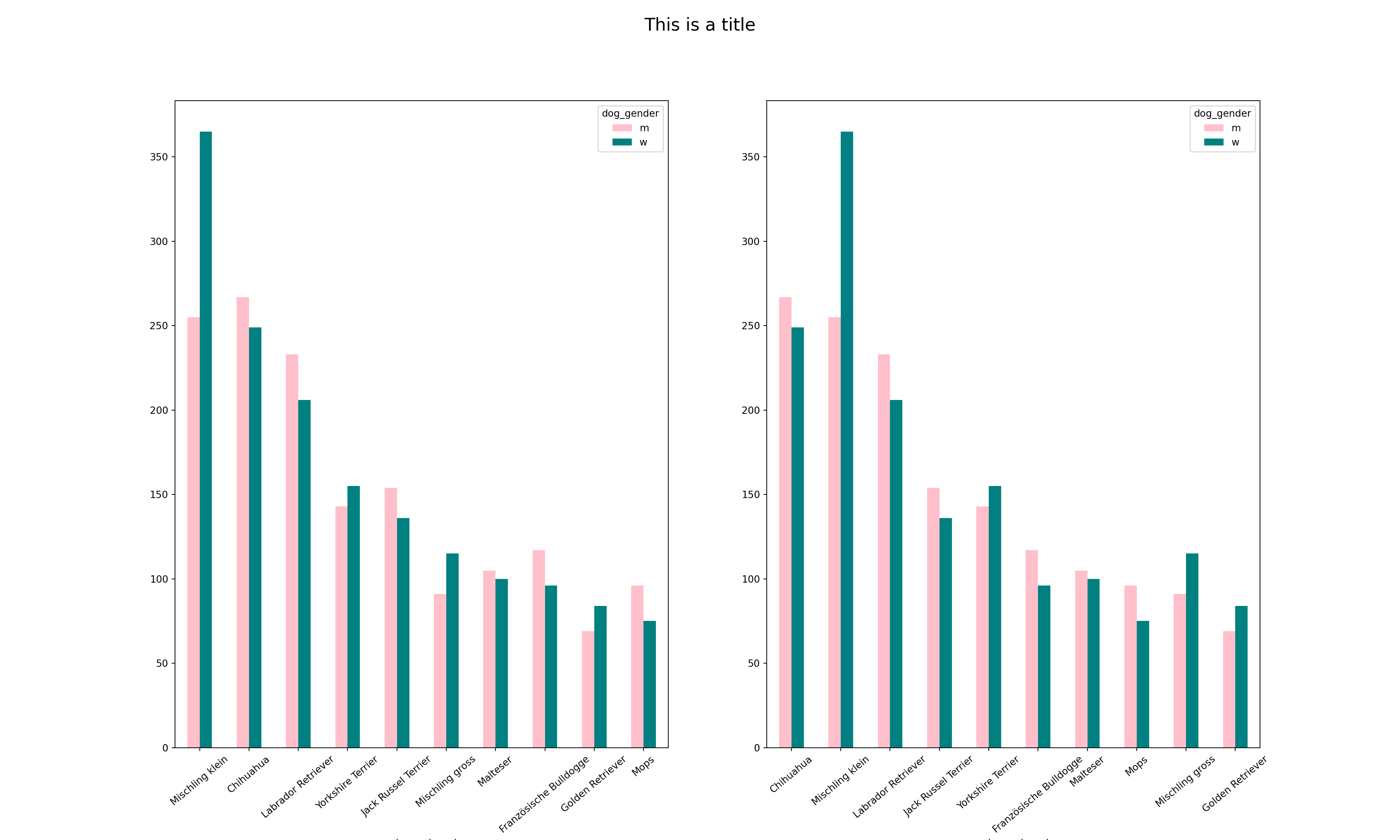
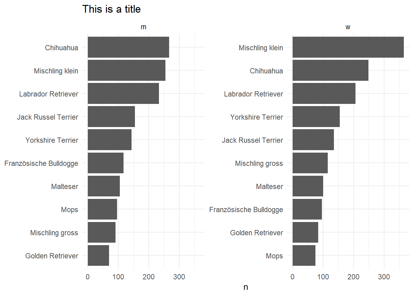
4. What are the top 10 most common primary breeds by dog gender? Visualize it using a bar plot
Python
main_table = df[['dog_gender','primary_breed']].pivot_table(index='primary_breed', columns='dog_gender', aggfunc=len).copy()


sorted_by_w = main_table.sort_values('w', ascending=False).head(10).copy()
sorted_by_m = main_table.sort_values('m', ascending=False).head(10).copy()


fig, axes = plt.subplots(1,2)

fig.suptitle("This is a title", fontsize=18)

sorted_by_w.plot(kind='bar', rot=40, color=["pink", "teal"], ax=axes[0], figsize=(20,12))
sorted_by_m.plot(kind='bar', rot=40, color=["pink", "teal"], ax=axes[1], figsize=(20,12))

R
dogs %>%
  count(dog_gender, primary_breed, sort = T) %>%
  group_by(dog_gender) %>%
  slice(1:10) %>%
  ggplot(aes(y = reorder_within(primary_breed, by =  n, within = dog_gender), x = n)) +
  geom_col() +
  facet_wrap(vars(dog_gender), scales = "free_y") +
  scale_y_reordered() +
  labs(y = NULL, title = "This is a title")+
  theme_minimal()

I start by counting the primary breed within each gender. I then visualize the data with ggplot2, leveraging the reorder_within, a function from tidytext to reorder the categories within each facet (gender). Alternatively we can remove the reorder_within and compare the primary breeds across gender instead of within.
5. Who (owner) has dogs with the largest age gap between them? What’s the gap value?
Python
df['dog_dob'] = pd.to_datetime(df['dog_dob'])
gb = df[['owner_id', 'dog_dob']].groupby('owner_id').agg([min, max])

gb.columns = ["_".join(list(x)) for x in gb.columns]

gb['diff'] = (gb['dog_dob_max']-gb['dog_dob_min']).dt.days

gb.sort_values('diff').tail(1)
##          dog_dob_min dog_dob_max  diff
## owner_id
## 87158     2000-04-10  2015-10-10  5661
R
dogs %>%
  group_by(owner_id) %>%
  filter(
    n() > 1,
    dog_dob == min(dog_dob) | dog_dob == max(dog_dob)
  ) %>%
  select(owner_id, dog_dob) %>%
  arrange(owner_id, dog_dob) %>%
  summarise(
    timediff = difftime(dog_dob, time2 = lag(dog_dob), units = "days")
  ) %>%
  fill(timediff, .direction = "up") %>%
  arrange(-timediff)
## # A tibble: 1,153 × 2
## # Groups:   owner_id [576]
##    owner_id timediff
##       <dbl> <drtn>
##  1    87158 5661 days
##  2    87158 5661 days
##  3    88250 5265 days
##  4    88250 5265 days
##  5   100112 5234 days
##  6   100112 5234 days
##  7   109472 4932 days
##  8   109472 4932 days
##  9   128461 4932 days
## 10   128461 4932 days
## # … with 1,143 more rows
I start off by filtering to owners having at least two dogs and take the oldest and youngest dog for each owner. I then arrange the dob within each owner’s group, calculate the difference between the ages and arrange by the difference in a descending order, giving us the owner with the largest gap.
During the session Adi Sarid suggested another solution, overall more concise and also to my liking. Instead of counting, filtering, etc., he suggests to straight up calculate the age differce between oldest and youngest dog and arrange that in a descending order:
dogs %>%
  group_by(owner_id) %>%
  summarise(age_gap = max(dog_dob) - min(dog_dob)) %>%
  arrange(desc(age_gap))
6. Save the Dataframe into an excel file where each sheet is a different age-group of owners
Python
writer = pd.ExcelWriter("dogs_by_owner_age_python.xlsx")

for age in df['age'].fillna("None").unique():
    temp_df = df[df['age']==age].copy()
    temp_df.to_excel(writer, sheet_name=age)

writer.save()
R
dogs %>%
  split(.$age) %>%
  writexl::write_xlsx(path = "dogs_by_owners_age.xlsx")
I really like here the use of split that splits a data frame into various lists by the variable passed to it. we can then use that – our object of data frames split by age – and pass it to write_xlsx that saves each element of the list as a sheet in our newly written .xlsx file.
That’s it, hope you enjoyed solving the questions. Make sure to checkout the recording!